Anatomical Record (The New Anatomist section), 257(6):195-207 (1999) [Wiley URL]
PROGRESS AND PERSPECTIVES IN
George Mason University, MS2A1, 4400 University Dr.- Fairfax, VA.22030-4444
Ph.: (703)993-4383; Fax: (703)993-4325; E-mail: ascoli@gmu.edu
Authors
mini-CV: Giorgio Ascoli is a faculty member of the Krasnow Institute
for Advanced Study and Visiting Assistant Professor in the Department of
Psychology at George Mason University. He received his Ph.D. in biochemistry
and neuroscience from the Scuola Normale Superiore of Pisa, Italy, and
has a long-standing interest in the neurobiological basis of consciousness.
After several years of experimental work at the National Institutes of
Health, Ascoli became interested in theoretical modeling and moved to Krasnow,
where he leads the Computational Neuroanatomy Group. His own contribution
to the research reviewed in this article is the result of a collaborative
effort with Stephen L. Senft (Krasnow Institute and Yale University) and
Jeffrey L. Krichmar (Krasnow Institute and The Neurosciences Institute).
Abstract. The tremendous increase in processing power of personal computers has recently allowed the construction of highly sophisticated models of neuronal function and behavior. Anatomy plays a fundamental role in supporting and shaping nervous system activity, yet to date most details of such a role have escaped the efforts of experimental and theoretical neuroscientists, mainly because of the problems complexity. When accurate cellular morphologies are included in electrophysiological computer simulations, quantitative and qualitative effects of dendritic structure on firing properties can be extensively characterized. Complete models of dendritic morphology can be implemented to allow the computer generation of virtual neurons that model the anatomical characteristics of their real counterparts to a great degree of approximation. From a restricted and already available experimental database, stochastic and statistical algorithms can create an unlimited number of non-identical virtual neurons within several mammalian morphological classes, storing them in a compact and parsimonious format. When modeled neurons are distributed in 3D and biologically plausible rules governing axonal navigation and connectivity are added to the simulations, entire portions of the nervous system can be grown as anatomically realistic neural networks. These computational constructs are useful to determine the influence of local geometry on system neuroanatomy, and to investigate systematically the mutual interactions between anatomical parameters and electrophysiological activity at the network level. A detailed computer model of a virtual brain that was truly equivalent to the biological structure could in principle allow scientists to carry out experiments that could not be performed on real nervous systems because of physical constraints. The computational approach to neuroanatomy is just at its beginning, but has a great potential to enhance the intuition of investigators and to aid neuroscience education.
Keywords: Dendrites,
L-Neuron, Modeling, Morphology, Neural networks, Simulations.
Rhyme and Reason
Over one hundred years ago, Ramon y Cajal proposed that the remarkable variety of neuronal shapes he was revealing with Golgi staining was a fundamental determinant of the biological activity of nervous systems30. Based on ample experimental evidence, modern neuroscientists have since widely accepted Cajals original intuition. Dendritic morphology plays an important role in the integration of synaptic inputs as well as in the back-propagation of action potentials. Axonal navigation mutually interacts with electrophysiological activity in dynamically shaping neuronal interconnectivity. Overall, network and cellular anatomy constitutes a crucial substrate of nervous system functions. Therefore, almost all aspects of neuroscientific investigation, from the system to the molecular level, need to take anatomy into full account.
The biological problem of neuroanatomy can be broadly summarized in the following questions:
(1) What is the best quantitative description of the geometry and topology of single neurons (in particular, neuritic morphology and development)?
(2) What is the influence of detailed dendritic morphology on the electrophysiological behavior of single neurons?
(3) How does axonal development determine (and how is it influenced by) network connectivity?
(4) What role do neuronal geometry and topology play on the emergent behavior of the neural system?
These questions are particularly challenging for current experimental technology. Procedures that allow the complete characterization of neurons from both the anatomical and physiological standpoint are extremely slow. The complete analysis of a handful of neurons by intracellular recording and dye filling for staining and reconstruction usually takes several weeks. On the other hand, when neurons are characterized only by anatomical or electrophysiological means, the key relationship between structure and activity cannot be established but by the statistical analysis of very large data sets.
This paper reviews the progress and perspectives of computational neuroanatomy, a nascent field of study that consists of the use of computer simulations to address the above fundamental neuroanatomical issues. Computational modeling can be of tremendous help in advancing our understanding of neuroanatomy for several reasons. The first one regards the ability to deal systematically and quantitatively with a very large parameter space. The investigation of the relationship between morphological parameters and neuronal electrophysiology and network connectivity has so far been a branch of descriptive biology. The leap from the present status to a quantitative description of the problem in the form of fundamental laws and equations is particularly arduous because of the large number of parameters involved. Such a difficulty becomes even more serious when one considers the great variability naturally occurring in both neuronal morphology and biochemistry, even within a specified cellular class.
Let us assume, for example, that we wanted to assess the influence of the number of dendritic bifurcations on the firing mode (e.g. simple versus complex spiking) of cerebellar Purkinje cells. We could depolarize and record the somatic membrane potential from a number of neurons within that class, and classify the firing mode given an identical stimulation protocol. Then we would proceed to tracing all those neurons so to count the bifurcations in their dendritic trees. Finally, we would establish the relationship (if any) between this morphological parameter and the electrophysiological behavior. This research design, however, would be frustratingly impractical, because too many other parameters are likely to affect the firing mode of Purkinje cells. These include, for instance, a non-identical distribution of active conductances throughout the dendrites of different individual neurons. A similar variability of many other morphological and biochemical parameters is also likely to affect firing mode and obscure the possibly minor effect of branch bifurcations. In order to carry out meaningful data analysis, an unthinkable number of experimental measurements should be taken.
Computational modeling, in contrast, can overcome this problem by allowing the systematic control of all parameters. Once the average morphological and physiological parameters of Purkinje cells are measured with just a few experiments, one could create a computer model of a Purkinje cell prototype. Then, while keeping the distribution of ionic channels and the other biochemical and morphological parameters constant, one could change the number of dendritic bifurcations and generate any number of virtual neurons which are identical in all aspects but for this particular parameter. It would then be immediately possible to analyze the influence of the bifurcation number on firing mode and to test how robust the result would be by repeating the simulations at different values of each of the other parameters. This logical procedure could be adopted to investigate systematically and quantitatively all aspects of the interplay between neuroanatomy and electrophysiology, but it also presents limitations that will be discussed in detail in the next section of this article. In general, computer simulations of combined neuroanatomical and neurophysiological models provide the speed and reliability necessary to explore systematically possible causal effects among all the parameters, and to suggest the design of specific wet experiments to confirm the quantitative correlations found.
A second important reason the computational approach could contribute to the progress in neuroanatomy is that direct visual observation and manipulation of 3-D structures in a graphic display or in virtual reality helps the development of novel intuitions among researchers and basic understanding among students. Even if detailed experimental observations remain the chief process underlying scientific discoveries, the complexity of nervous system anatomy requires the assembly of theoretical models in order to maintain an integrated perspective. If we were able to build a complete virtual model of (a part of) the nervous system, and this model displayed all the emergent properties that could be observed in the biological counterpart, then this would constitute a positive indication that our knowledge of the real system would be nearly complete. If, on the other hand, we were not able (due to technical limits) to measure all the necessary parameters to build a complete model, then searching the space of missing parameters for sets of values that could reproduce experimental measurements of other emergent parameters would represent a valid alternative strategy. (The term emergent, referred to the parameters or properties of a model, is used here and in the rest of this review to indicate those aspects of the model that were not trivially and directly built in, and that can be thus used to test or verify the correctness of the model itself.) Finally, if we were only able to build partial models of neuroanatomical systems, these would still prove useful to summarize and organize our knowledge, and to suggest the most important directions of the next stage of research.
The computational approach can become most efficient if both physiological and anatomical details are included. Most computer models of neuronal function are currently limited to the biochemical and biophysical bases of electrophysiology. However, nervous systems are too complex, and the role of neuronal structure and network connectivity is too pervasive, for neuroanatomy to be approximated away in biologically plausible models. In future perspective, the integration of all fundamental aspects of neuroscience is likely to be necessary to generate accurate virtual brains in computer software.
Historically, modern neuroscience started with neuroanatomy. Through the work of Golgi, Cajal, Lorente De No, and other pioneers, neuroanatomy had become a coherently developed and deeply understood science well before the appearance of electrophysiology and molecular biology. Neuroanatomical data have been continuously collected for over a century and particularly in the last few decades, resulting in thousands of quantitative and qualitative publications, and in a large number of neuronal tracings accumulated in laboratories throughout the world. Despite this wealth of data, neuroanatomical modeling is not as common an approach as electrophysiological modeling. This may be due in part to the fact that neurophysiological activity can be represented in computer models by the relatively intuitive mathematical formalism of electrical circuits. In contrast, it is difficult to accurately describe and convey the physical complexity of neuroanatomical structures by differential equations. The breathtaking advancement that computer graphic technology has achieved in recent years, however, offers a valid alternative to an abstract mathematical representation. Neuroanatomical rules can be implemented in algorithms to generate virtual three-dimensional structures, and these can be stored and analyzed much like their real counterparts, namely as a list of neuritic compartments and connectivity.
Neuroscientists have just started appreciating this new approach, and computational neuroanatomy is currently in its nascent stages. The interest in this field, however, is growing rapidly, and it seems safe to predict that the present and future collaborative effort of neuroanatomists and computer scientists will bring an essential contribution to the advancement of neuroscience.
The next
sections of this review describe the state of the art of three extremely
promising applications of computational neuroanatomy: the analysis of the
effect of dendritic structure on a single neuron electrical activity, the
generation and description of dendritic morphology, and the anatomical
modeling of biological neural networks.
Relationship between structure and activity in single neurons
There are several non-exclusive theories to explain the peculiar tree-like shape of neuronal dendrites. A simple hypothesis is that the branching structure might be the most efficient shape to invade the surrounding space and maximize the inputs received, given physical and metabolic constraints10. Researchers have also proposed that, because the soma integrates dendritic inputs in a highly nonlinear fashion, the variable dendritic path length from synapses to the soma could act as a delay line, allowing precise time computations and coincidence detection1. In addition, the discovery that dendrites can transmit electric impulses by active conductance19, and that the action potential can back-propagate from the soma throughout the dendritic tree34, opened the possibility that specific morphological characteristics of dendrites have precise effects on neuronal computation. Are there so many different morphological classes of neurons because each of them is particularly suitable to carry out a specific computational task? Similarly, within a morphological class, do geometrical and topological differences among individual neuron affect the electrophysiological behavior of single cells?
From Ohms law and cable equation, it is expected that, as the dendritic surface increases, a higher input conductance would result in lower excitability. This means that, given an identical distribution of biochemical machinery and the same stimulation protocol, smaller cells should display higher firing rates. So far only few studies have investigated the relationship between dendritic morphology and single-cell electrophysiology, and they mainly focussed on the firing mode, i.e. whether a cell spikes (fires a regular sequence of action potentials) or bursts (fires action potentials grouped in trains).
Studies in the cortex showed that cells in layer 5 were more likely to burst if the apical dendrites were thick, and spike if the apical dendrites were slender22. Similarly, it was observed that CA3 pyramidal cells tended to burst as the length of the apical dendrite increased5. A more recent simulation study showed that, given an identical distribution of ionic channels across different cortical cell types, smaller cells (stellate cells) generally spiked, whereas larger cells (pyramidal cells) tended to burst24. These results can be explained in part by a previous computational model suggesting that the spiking versus bursting behavior critically depends on the ratio of somatic surface to dendritic surface27.
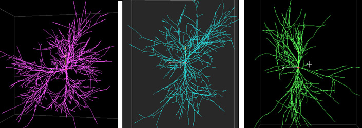
Only recently did researchers start analyzing systematically and extensively the quantitative and qualitative effect of morphological parameters on neuronal firing. This effort was made possible by the public release of electronic archives of dendritic morphology, i.e. collections of hundreds of computerized neuronal tracings. Using one such archive (particularly, the Southamptons8), Krichmar and coworkers21 loaded several CA3 pyramidal cells with a standardized distribution of ionic conductances and concentrations37, and ran simulations by stimulating the neurons with a uniform somatic injection of depolarizing current. The result was an extremely wide range of responses by the modeled neurons, both in terms of firing mode (spiking versus bursting) and firing rate21. The electrophysiological response of neurons is expected to be highly sensitive to changes in membrane properties, ionic distributions, and amount and mode of excitation. In Krichmars models, however, all these parameters were set identical for all cells, and the only differences concerned the dendritic morphology (Fig. 1). These results are even more intriguing in that the simulated neurons belonged to the same morphological class, therefore their structural variability was not extreme.
Modeling dendritic morphology
The above results demonstrate that computational models of neuronal behavior should be anatomically realistic in order to be physiologically plausible. The number of neurons available in electronic archives, however, is limited. Currently available microprocessors allow neuroscientists to model the electrical activity of entire networks composed of many anatomically complete neurons. At the present rate of increase of computational power, and with no techniques available to acquire additional neuronal tracings in a fast and efficient manner, the simulation capacity of computers will soon outgrow experimentally available neuroanatomical data. A natural solution to this problem is to model neuronal morphology, i.e. to generate virtual neurons that are anatomically equivalent to the real ones.
One of the first steps in this direction was moved in the late seventies by Hillman14. He proposed that a series of quantitative neuroanatomical correlations could completely describe the dendritic morphology of any neuron with a set of fundamental parameters. For example, the relationship between the diameter of a dendritic branch before a bifurcation and the diameters of the two stemming branches could be described by Ralls power rule29. This rule states that the sum of the daughter branches diameters elevated to a certain power equals the parent branchs diameter elevated to the same power. According to Hillman, Ralls power is one of the fundamental parameters, and varies depending on the morphological class of the neuron. Similarly, the ratio of the two daughters diameters is also a fundamental parameter, with a range of values typical of a morphological class. Hillman maintained that, in principle, an entire dendritic tree could be described recursively by analyzing the local morphology of branches15. This means that geometrical parameters (e.g. the branch length from a stem or a bifurcation to the next bifurcation or termination point) and topological parameters (e.g. the probability of a branch to end in a bifurcation or in a termination point) are postulated to correlate with purely local constraints such as the branch diameter.
- Measure the statistical distributions of fundamental parameters (i.e. the parameters used by the descriptive algorithm) from an experimental data set of dendritic morphology.
- Use these distributions as the input to L-Neuron and generate a set of virtual neurons. Translate these output neurons in a format analogous to that of the experimental data set.
- Compare real and virtual neurons. Clearly, the distributions of fundamental parameters will be identical. However, the statistical distributions of all the morphological parameters not used trivially in the descriptive algorithm (the emergent parameters) can be used to characterize the plausibility of virtual neurons. If virtual and real neurons are statistically indistinguishable, the descriptive algorithm is deemed accurate.
- If there are discrepancies between real and virtual neurons, their analysis can be helpful to modify and improve the descriptive algorithm (i.e. to find better anatomical rules). Once the new L-Neuron algorithm is re-implemented, repeat the procedure from #2.
The L-Neuron project has demonstrated that the stochastic and statistical implementation of recursive neuroanatomical algorithms is a promising approach to generate virtual models of dendritic morphology based on experimental data. Additional neuroanatomical rules have been proposed to capture quantitative aspects of neuronal structures. For example, based on theoretical considerations, specific morphological parameters can be correlated with one another in order to optimize volume occupation. Specifically, the average dendritic bifurcation angle was predicted (and, for many neuronal species, observed) to correlate with the average daughter-to-parent area ratio11. Based on similar considerations of volume optimization, the range of values for Ralls power parameter was found to be restricted in axonal branching25. Models can also be improved by adding a dependency of the bifurcating probability on the distance grown from the previous bifurcation26. These and other neuroanatomical rules or empirical observations will be added and tested in future L-Neuron implementations during the search for the most accurate and general algorithm.
A different approach to modeling dendritic morphology consists of constraining the topological parameters (mainly, the bifurcating probability) to the global (as opposed to the local) position within the tree, and particularly to the order of branching. This strategy can also be implemented in a stochastic and statistical fashion, and can take into account systematic components of local interaction as well9. Among the most influential proponents of the above principles, van Pelt and coworkers developed several growth models at different levels of complexity, that reproduced a great deal of observed morphological characteristics of dendritic trees (as recently reviewed40). In the simplest scenario, the probability of a terminal branch to elongate is set to decrease exponentially with its order (i.e. with its distance from the soma measured in number of intervening bifurcations). The probability of non-terminal branch to elongate (that is, to give rise to a bifurcation) is complementary to the terminal probability. In addition to these two simple parameters (the rate of exponential decrease and the ratio of terminal vs. non-terminal growth), more complex models of this kind take into account the variability of the total number of dendritic segments and the distribution of growth events (i.e. the attachment of new branches) in time40.
Anatomically accurate neural networks
In the topological models of neuronal morphology, neuritic segments are attached to growing tips of dendrites, which compete with each other for new additions. This principle has been successfully extended to a population-based growth algorithm, designed and implemented by Senft in a program called ArborVitae31. The crucial observation is that the anatomical characteristics of single neurons, dendrites, and axons, can be quantitatively derived and described by pooling all individual structures in groups33. In ArborVitae, dendrites are distributed to the growing tips of a group of neurons, rather than to individual cells. This approach reflects a competition for metabolic resources among all neuronal members of a population. This strategy also achieves a tremendous computational efficiency, because it describes and generates neurons class by class (as opposed to L-Neuron that describes morphological classes, but within them generates single individuals one by one). In one sweep, ArborVitae can generate any number of neurons within a class by dealing all the dendrites available for that group to the whole set of somata at once31.
The dealing of dendrites in ArborVitae occurs in four consecutive phases. In the appending mode, dendritic segments are distributed to somata or to the previous dendritic group (e.g. distal dendrites are attached to proximal dendrites). In the first extending phase, segments are attached to the stems of their own groups or to the terminal tips of other extending dendrites, causing the elongation of the tree. The branching phase consists in the distribution of segments to non-terminal points of the same dendritic group. The last phase is a second turn of extending attachment32. More complex dendritic topologies can be simulated by growing several distinct groups of dendrites in consecutive layers of the tree (e.g. proximal segments, lateral segments, distal segments, etc.).
Similarly to the models described in the previous section, ArborVitaes algorithms sample values of geometrical parameters (angles, diameters, etc.) stochastically within statistical distributions. In addition to describing neuronal morphology and growth in time, however, Senfts program addresses the issue of the space distribution of neurons. Since neurons are grown in groups, the statistical description (and generation) of their geometry also results in overall system (or tissue) anatomical properties. Neurons can thus be arranged in nuclei, laminae, or variously shaped layers.
As neurons grow in space, axons search for their targets guided by gradients of neurotrophic factors. Because both axons and their targets are described as populations, ArborVitae naturally implements a model of axonal navigation that is also statistical and stochastic32. Axons select their targets and grow toward them, allowing synaptic connections to be established. The same general algorithm for axonal outgrowth can simulate (with the appropriate parameter values) such different navigations modes as recognized in perforant pathways, climbing fibers, and isotropic sprouting.
Examples of recently implemented ArborVitae networks include the thalamo-cortical connections31, the hippocampal tri-synaptic circuit2, and a larger scale of the rat CA1 region32 (Fig. 6). In principle, once the neuronal morphology and the network wiring are both developed, electrophysiological simulations can be run on the entire system. Unfortunately, the computational tools currently available for electrophysiological modeling are not powerful enough to allow a practical simulation of the active conductance throughout a network of many million compartments. Consequently, medium- and large-scale ArborVitae outputs can be either downloaded to files and used for off-line neurophysiological simulations, or loaded with a simplified passive conductance model to run on-line within the ArborVitae environment.
Ideally, the simulation of anatomical development and electrophysiological activity should be part of a single integrated model, to reflect the deep reciprocal bond between structure and activity underlying neurobiological dynamics. Network connectivity clearly affects the electrical behavior of neurons, and at the same time, axonal navigation is influenced by the underlying electrophysiological activity. So far, only abstract studies have been carried out to investigate the influence of dendritic outgrowth on network activity38. In order to establish firm and quantitative correlations between network anatomy and emergent behavior, one should expand these abstract models to incorporate anatomically and physiologically plausible computations. At present, the major limitation towards such a complete model is constituted by the difficulty to reduce the computationally intensive compartmental simulations of large-scale neuronal electrophysiology to a more tractable formalism. Interestingly, while only few researchers have attempted to develop more efficient electrophysiological formalisms20, the computational description of network anatomy starting from single-cell morphology can already generate structures with thousands of neurons on low-cost computers.
The complexity
of neuronal anatomy and of the ArborVitae models makes the quantitative
comparison of virtual and real networks a slow and challenging process,
that has just begun. The ArborVitae algorithms for neuronal network development
use hundreds of parameters (as opposed to the handful used for single-neuron
growth by L-Neuron or van Pelts models), and the investigation of their
effects and roles requires an elaborated statistical analysis. However,
the above results show that the computer generation of anatomically accurate
neural networks is not an impossible task to achieve in the near future.
This line of research carries the potential to investigate many fundamental
issues, such as the influence of dendritic morphology on network connectivity
and emergent behavior.
Conclusions and future directions
The human brain is reportedly the most complex object in the Universe, and its product human cognition is among the most fascinating and mysterious intellectual challenges to scientific understanding. It is not a shame to admit that we do not yet understand how higher cognitive functions arise from the nervous systems. From a materialistic point of view, the safest way to reproduce a process analogous to human consciousness into a computer is to build a complete model of the brain. It is known that anatomy plays a crucial role in brain function and development, yet the details and limits of this role are hard to grasp and define. Therefore, we submit that computational neuroanatomy could be pivotal, in the long term, to understand the connection between the mind and the brain.
The computational neuroanatomical studies reviewed in the first section of this paper showed that detailed dendritic morphology dramatically affects single cell electrophysiology. Further investigation is needed to address whether the quantitative and qualitative results obtained so far are specific for one morphological class (CA3 pyramidal cells) and one physiological model (Traubs), or reflect a more fundamental relationship between neuronal structure and activity. Many more fundamental questions await extensive investigation: what is the influence of detailed neuronal morphology on network connectivity? What is the effect of detailed network connectivity on the emergent network behavior and the resulting computation?
In order to address these issues, the computational approach seems particularly promising, in that it makes it possible to carefully control the large number of parameters involved. Two strategies have been described that allow the generation of virtual neuronal structures as an aid for modeling. L-Neuron is a relatively simple tool that implements recursive sets of local rules, such as Hillman/Tamoris or Burkes. In L-Neuron, geometric parameters consist of statistical distribution of experimental measurements of dendritic morphology, with a minimum amount of best fitting required. Consequently, it is relatively straightforward to obtain feedback on the accuracy of the growth algorithm by comparing the emergent structure of virtual and real neurons. ArborVitae is a more complex and ambitious project that implements topological (van Pelt-like) algorithms on a population basis, and allows the computationally efficient generation of neuronal network anatomy. ArborVitae makes use of a large number of fundamental parameters, many of which cannot be measured simply and directly from experimental data. Therefore, novel automatic analysis utilities are being implemented to exploit the full potential of the program.
Among the most important variables leading to the complexity of neural function is synaptic connectivity. While this issue is not directly pertinent to the L-Neuron project (that only deals with single cells), synaptic connectivity is modeled in ArborVitae. It is important to underline here that biological network connectivity adds a tremendous challenge to computational neuroanatomy for three reasons. First, axonal morphology is more difficult to trace than dendritic morphology, mainly because of the length of the neuritic processes. Second, the quantitative measurement of the connectivity parameters (e.g. number, type, and distribution of synapses; specificity and selectivity of the connections among different morphological classes of neurons) is extremely difficult, and experimental data are only available for a few brain regions (such as the hippocampus32). Third, the number of synaptic connections established by each neuron of the network is very large. Consequently, it becomes very problematic to analyze the physiological and computational effects of specific connectivity parameters. ArborVitae should be viewed as one of the first available tool for the computational neuroscience community to start approaching these problems.
Both L-Neuron and ArborVitae implement stochastic sampling, which allows many non-identical neurons to be generated from one set of statistical distributions (i.e. from one morphological class description). This feature results in a tremendous potential for data compression, data amplification, and biological plausibility. On the other hand, once neurons (or networks) are generated, they can be archived individually in the traditional Cartesian format, specifying the position in space and the connectivity of each dendritic, axonal, or somatic element. The level of description of L-Neuron and ArborVitae, therefore, can be expanded in principle to incorporate electric conductance and capacitance, neurotransmission, and any further compartmental property, such as microtubule dynamics, activity and sub-cellular localization of enzymatic components, concentration and diffusion of chemicals, gene transportation, and so forth. Naturally, at this stage of progress the computational power of standard computers practically limits the depth of the models features. However, it is encouraging to report that the anatomical characteristics of small portions of a mammalian brain (a hippocampal slice) can be reproduced accurately, and the electrophysiological activity of such a network can be in principle simulated off-line and loaded back to the network for display and analysis.
L-Neuron runs under DOS on Pentium-class processors, and can generate thousands of neurons in seconds. ArborVitae currently runs on Silicon Graphics machines, and can grow a complete interconnected million-compartment network in less than ten minutes on an O2 computer. It is easy to predict that as more and more powerful computers become available at affordable prices, the computational approach to neuroanatomy will become an invaluable aid to research and education. Within a decade or two, an anatomical computer model might be constructed for the entire rat brain. A model of this sort would likely contain many untested assumption, but its own internal consistency could lead to important hypotheses and ideas. The potential applications (and implications) of such a virtual brain would be phenomenal.
Neuroanatomists are traditionally less prone towards mathematical modeling and computer simulations than electrophysiologists. The future progress of computational neuroanatomy is critically bound to the development of user-friendly computer interfaces, which will guarantee an extensive diffusion and usability of software such as L-Neuron and ArborVitae by the neuroscientific community. Ease of use and intuitive understanding are challenging to accomplish together with biological accuracy and quantitative analysis. This effort will be useful to address the issue of format standardization in quantitative neuroanatomy. L-Neuron can extract statistical data from a variety of experimental and archive formats (such as Southamptons CellViewer8, Neurolucida12 and Eutectic-like17), and ArborVitae can graphically display these structures directly. Both L-Neuron and ArborVitae can output files for neurophysiological simulators such as Genesis6 and Neuron16, as well as for each other and for CellViewer. The diffusion of this software will thus help neuroscientists store, exchange and compare experimental and modeling data in electronic form.
Science traditionally advances by means of experimental discoveries that are subsequently interpreted within a theoretical framework (possibly built around them), or by means of theoretical predictions in the context of an existing model that are subsequently verified experimentally. Electrophysiology is currently at a stage where experimental progress (e.g., discovery and characterization of new ionic channels, and biochemical analysis of their control and regulation) and computational modeling (compartmental simulations of electric conductance) advance in parallel. This synergy is particularly evident at the network-to-system level. In a typical chain of studies18, neuronal oscillation at specific frequencies are discovered and characterized in a brain region; network simulations are built using appropriate single-neuron models, and the model parameter are set so to reproduce the oscillations; simulations suggest a variety of implications regarding the nature of the oscillations (for instance, that they are driven by inhibitory interneurons); and finally, the simulation predictions are verified experimentally (e.g., by inhibiting the interneurons and observing the consequent lack of oscillations). It is the entire set of studies that yields a complete understanding of the cellular basis of the phenomenon of these oscillations.
Neuroanatomy is
in a strikingly contrasting situation, with a century of quantitative data
accumulated and little or little modeling effort to summarize and rationalize
them. The availability of inexpensive computers of sufficient power to
run simulations such as those described in this review constitutes a tremendous
opportunity to catch up with the experimental knowledge, and to push progress
forward from both the theoretical and the empirical side. The incorporation
of quantitative anatomy within our computational and intellectual model
of nervous system function represents a critical step towards the generation
of a truly accurate virtual brain.
Acknowledgments:
I am deeply indebted to my collaborators Drs. Stephen L. Senft (Krasnow
Institute and Yale University) and Jeffrey L. Krichmar (Krasnow Institute
and The Neurosciences Institute). With them I share the merit of my work
on computational neuroanatomy, including the contribution of our group
to the results reviewed in this paper. I also wish to thank Dr. James L.
Olds (Krasnow Institute) for critically reviewing this manuscript and for
his continuous encouragement and support. This work was supported in part
by Human Brain Project grant R01-NS39600-01 by the National Institute of
Neurological Disorders and Stroke (National Institutes of Health) and by
Award No. 00-1 from the Commonwealth of Virginias Alzheimers and Related
Diseases Research Award Fund, administered by the Virginia Center on Aging,
Virginia Commonwealth University.
Citations and References
1. Agmon-Snir H, Carr CE, Rinzel J. 1998. The role of dendrites in auditory coincidence detection. Nature. 393(6682):268-272.
2. Ascoli, GA, Hunter L, Krichmar JL, Olds JL, Senft SL. 1998. Computational neuroanatomy of the hippocampus. J Neurosci (Suppl) 24(806.10):2015.
3. Ascoli GA, Krichmar JL. 1999. L-Neuron: a modeling tool for the efficient generation and parsimonious description of dendritic morphology. Neurocomputing, In Press.
4. Ascoli GA, Krichmar JL, Olds JL, Hunter L, Senft SL. 1997. Computer generation of sets of anatomically plausible neurons for modeling. J Neurosci (Suppl) 23(645.5):1674.
6. Bower JM, Beeman D. 1998. The Book of GENESIS: Exploring Realistic Neural Models with the GEneral NEural SImulation System. New York: Springer-Verlag.
7. Burke RE, Marks WB, Ulfhake B. 1992. A parsimonious description of motoneurons dendritic morphology using computer simulation. J Neurosci 12(6):2403-2416.
10. Caserta F, Hausman RE, Eldred WD, Kimmel C, Stanley HE. 1992. Effect of viscosity on neurite outgrowth and fractal dimension. Neurosci Lett 136(2):198-202.
11. Cherniak C. 1992. Local optimization of neuron arbors. Biol Cybern 66(6):503-510.
12. Glaser JR, Glaser EM. 1990. Neuron imaging with Neurolucida--a PC-based system for image combining microscopy. Comput Med Imaging Graph 14(5):307-317.
13. Hamilton P. 1993. A language to describe the growth of neurites. Biol Cybern 68(6):559-565.
14.Hillman DE. 1979. Neuronal shape parameters and substructures as a basis of neuronal form. In Schmitt F (ed): The Neurosciences, Fourth Study Program Cambridge, MA: MIT Press, p. 477-498.
15.Hillman DE. 1988. Parameters of dendritic shape and substructure: intrinsic and extrinsic determination? In Lasek RJ, Black MM (eds): Intrinsic Determinants of Neuronal Form and Function. New York: Liss, p. 83-113.
16. Hines ML, Carnevale NT. 1997. The NEURON simulation environment. Neural Comput 9(6):1179-1209.
17. Jacobs GA, Nevin R. 1991. Anatomical relationships between sensory afferent arborizations in the cricket cercal system. Anat Rec 231(4):563-572.
18. Jefferys JG, Traub RD. 1998. Electrophysiological substrates for focal epilepsies. Prog Brain Res 116:351-358
19. Johnston D, Magee JC, Colbert CM, Cristie BR.1996. Active properties of neuronal dendrites. Annu Rev Neurosci 19:165-186.
20. Krichmar JL, Ascoli GA, Hunter L, Olds JL. 1997. A model of cerebellar saccadic motor learning using qualitative reasoning. Lecture Notes Computer Science 1240:134-145.
21. Krichmar JL, Washington SD, Ascoli GA. 1999. Effect of dendritic morphology on CA3 pyramidal cell electrophysiology. Submitted.
22. Larkman A, Mason A. 1990. Correlations between morphology and electrophysiology of pyramidal neurons in slices of rat visual cortex. J Neurosci 10(5):1407-1414.
23. Lindenmayer A. 1968. Mathematical models for cellular interaction in development I&II. J Theor Biol 18:280-315.
24. Mainen ZF, Sejnowski T. 1996. Influence of dendritic structure on firing pattern in model neocortical neurons. Nature 382:363-366.
25. Mitchison G. 1991. Neuronal branching patterns and the economy of cortical wiring. Proc R Soc Lond B Biol Sci 245(1313):151-158.
26. Nowakowski RS, Hayes NL, Egger MD. 1992. Competitive interactions during dendritic growth: a simple stochastic growth algorithm. Brain Res 576(1):152-156.
27. Pinsky PF, Rinzel J. 1994. Intrinsic and network rhythmogenesis in a reduced Traub model for CA3 neurons. J Comput Neurosci 1(1-2):39-60.
28. Prusinkiewicz P, Lindenmayer A. 1990. The Algorithmic Beauty of Plants. New York: Springer-Verlag.
29. Rall W. 1959. Branching dendritic trees and motoneurons membrane resistivity. Exptl Neurol 1:491-527. Reprinted in Segev I, Rinzel J, Shepherd GM (eds.): The Theoretical Foundation of Dendritic Function. Cambridge MA: M.I.T. Press, 1995, p. 37-73.
30. Ramon y Cajal S. 1894-1904. Textura del Sistema Nervioso del Hombre y los Vertebrados. 1994 English translation by N. and L.W. Swanson, Oxford University Press.
31. Senft SL. A statistical framework to present developmental neuroanatomy. In Donahoe J (ed): Biobehavioral Foundations Elsevier Press.
32. Senft SL, Ascoli GA. 1999. Reconstruction of brain networks by algorithmic amplification of morphometry data. Lecture Notes Computer Science 1606:25-33.
33. Senft SL, Woolsey TA. 1991. Computer-aided analyses of thalamocortical afferent ingrowth. Cerebr Cort 1:336-347.
34. Stuart G, Spruston N, Sakmann B, Hausser M. 1997. Action potential initiation and backpropagation in neurons of the mammalian CNS. Trends Neurosci 20(3):125-131.
35. Symanzik J, Ascoli GA, Washington SD, Krichmar JL. 1999. Visual data mining of brain cells. Comp Sci Stat, In Press.
36. Tamori Y. 1993. Theory of dendritic morphology. Phys Rev E 48(4):3124-3129.
37. Traub RD, Jefferys JGR, Miles R, Whittington MA, Toth K. 1994. A branching dendritic model of a rodent CA3 pyramidal neurone. J Phys 481.1:79-95.
38. van Ooyen A, van Pelt J. 1996. Complex periodic behaviour in a neural network model with activity-dependent neurite outgrowth. J Theor Biol 179(3):229-242.
39. van Pelt J. 1997. Effect of pruning on dendritic tree topology. J Theor Biol 186(1):17-32.
40. van Pelt J, Uylings HBM. 1999. Natural variability in the geometry of dendritic branching patterns. In Poznanski RR (ed): Modeling in the Neurosciences From Ionic Channels to Neural Networks. Amsterdam (The Netherlands): Harwood Academic Publishers, Chap. 4, p. 79-108.
41.
Washington SD, Ascoli GA, Krichmar JL. 1999. Statistical Analysis of Dendritic
Morphology's Effect on CA3 Pyramidal Cell Electrophysiology. Neurocomputing,
In Press.
Figures
Figure 1. Effect of dendritic morphology on neuronal electrophysiology.
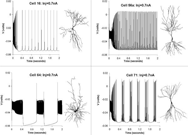
Reconstructed
CA3 pyramidal cell from electronic archives (www.neuro.soton.ac.uk/cells/cellArchive.html)
were converted to Genesis descriptor files. Somata and axons were substituted
by the same compartments in all cells, and the Traub model was loaded using
an identical distribution of physiological parameters for all neurons.
When the same 0.7 nA current was continuously injected in the soma of several
cells, different firing patterns were obtained. These dramatic differences
are thus uniquely due to the variation in dendritic structure among cells.
Three distinct firing modes are apparent in these examples: regular spiking
(cells 16 and 56a), plateau bursting (cell 64), and regular bursting
(cell 71). Quantitative differences such as spiking frequency in cells
16 and 56a are also due to different dendritic morphologies. Results by
the author and Jeff Krichmar.
Figure 2. Hillmans algorithm.
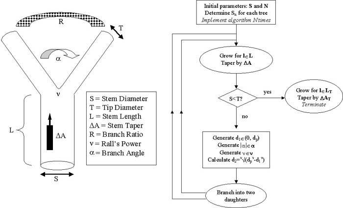
Dendritic
morphology can be described with a set of local rules determining the geometrical
behavior of branching. A branch grows for a certain length (L) while
tapering (DA), and then it bifurcates
or terminates depending on the final diameter and a diameter threshold
(T). If the branch bifurcates, it stems two daughter branches at
an angle a, with diameters determined
by a ratio (R) and Ralls power n.
Since the two new stems behave like the original branch, this algorithm
is recursive, as schematized by the flow chart.
Figure 3. A virtual Purkinje cell generated by L-systems.
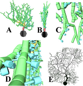
The
cell modeled in panels A-D was created with only 11 lines of stochastic
L-system to resemble the real 2107-compartment Purkinje cell shown in panel
E (from www.ls.huji.ac.il/~rapp/reconst.html). Spines (in blue) were added
within the L-systems description but were not present in the experimental
file. A: Front view; B: side view (note the quasi-planarity typical of
this morphological class); C: detail on dendritic branches; D: detail on
dendritic spines. Partially adapted from reference 4.
Figure 4. A screenshot from L-Neuron.
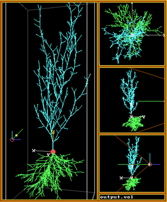
The main panel displays a virtual pyramidal cell grown with Tamoris algorithm, using experimental data provided by Hillman for cortical neurons14. Basal dendrites are color-coded in green, apical dendrites in blue, and the soma in red. The side views represent the same cell in different perspectives from the top (top panel), front (middle panel) and side (bottom panel).
Figure 5. The basic L-Neuron algorithms.
These motoneurons were simulated using the algorithms by Hillman (green, left), Tamori (blue, center), and Burke (red, right). In Hillmans models, diameters are calculated with Ralls power rule, while angles are measured empirically. In Tamoris model, both diameters and angles are calculated. In Burkes model, both diameters and angles are measured empirically.
Figure 6. ArborVitae simulations of the rat hippocampal slice.
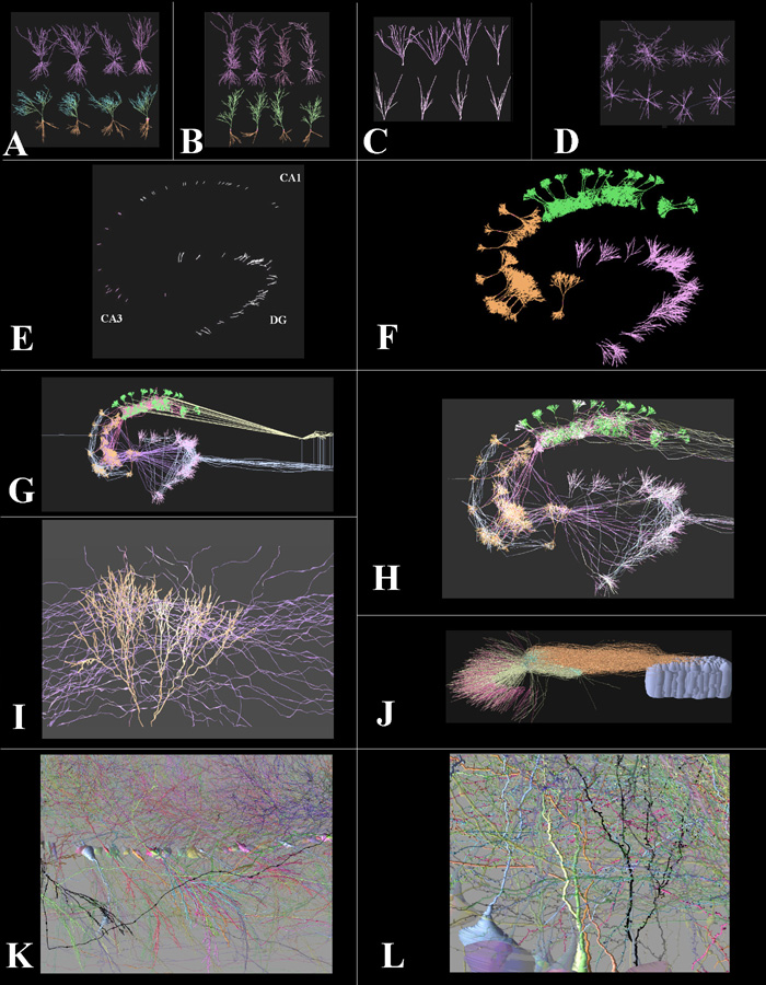
The
four main classes of hippocampal neurons were each modeled as a distinct
morphological group: CA3 pyramidal cells (A), CA1 pyramidal cells (B),
dentate granule cells (C) and polymorphic interneurons (D). Real cells
(four examples shown in the top rows of A-D) were used to obtain the parameters
used to generate virtual cells (four examples shown in the bottom rows
of A-D). A-B: basal dendrites are in brown and apical dendrites are in
green. E: a small-scale network model2 with approximately 50
cell bodies distributed in space according to the typical lamellar curvature
of CA3, CA1 and the dentate gyrus (DG). F: dendrites were then distributed
within each region (CA3 in brown, CA1 in green, DG in purple). The addition
of black-box entorhinal columns (right) and a septo-hippocampal pathway
module (left) provided the network input/output loop. The network was then
wired by the axonal connectivity (G), and passive current propagation was
simulated (H, white color indicates depolarized membrane). I: a detail
of apical dendrites in CA3 with incoming axonal fibers. J: a larger network
for the CA1 region32, with approximately 5000 neurons. K: a
simulation of Golgi staining (only showing ~1% of neuronal structures),
displaying several somata lined in the pyramidal layer, with apical dendrites
on the top and basal dendrites (plus a transversal axonal fiber in black)
on the bottom. Each pyramidal cell was given a different color, making
it possible to follow the dendritic trees stemming from individual neurons.
L: an enlargement with several dendritic spines visible. Partially adapted
from references 2 and 32. Results by the author and Steve Senft.